I wanted to share a quick tip on creating sine/sinusoidal functions in Femap. Some people set these up in Excel first and paste them in from the clipboard, but this will explain how to avoid using that second program. We’ll be setting up functions to describe the time history of a dynamic load for modal transient response (SOL112 aka “3..Transient Dynamic/Time History”) analysis.
A sinusoidal time history signal can be of the form Asin(ωt+φ), where A = amplitude, ω = angular/circular frequency, and φ = phase angle, the last of which is usually ignored as we’ll simply start from 0deg.
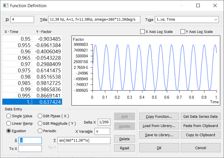
To create 1 second of loading at 11.39 hz with 200 increments, enter Femap’s Function Definition dialog, select “Equation”. Then,
- X = start time = 0
- To X = end time = 1
- Delta X = time increment = 1/200
- Leave X Variable as “x”
- Enter the sine function for Y = sin(360*11.39*!x). This is the tricky part; Femap expects deg/s. Also, Femap’s equation functionality expects a “!” in front of the variable.
In the image below, I have already selected “Add”, so the function is viewable. Femap resets the X to the previous To X, and To X to blank as it wants to assist you with optionally appending to the time history.
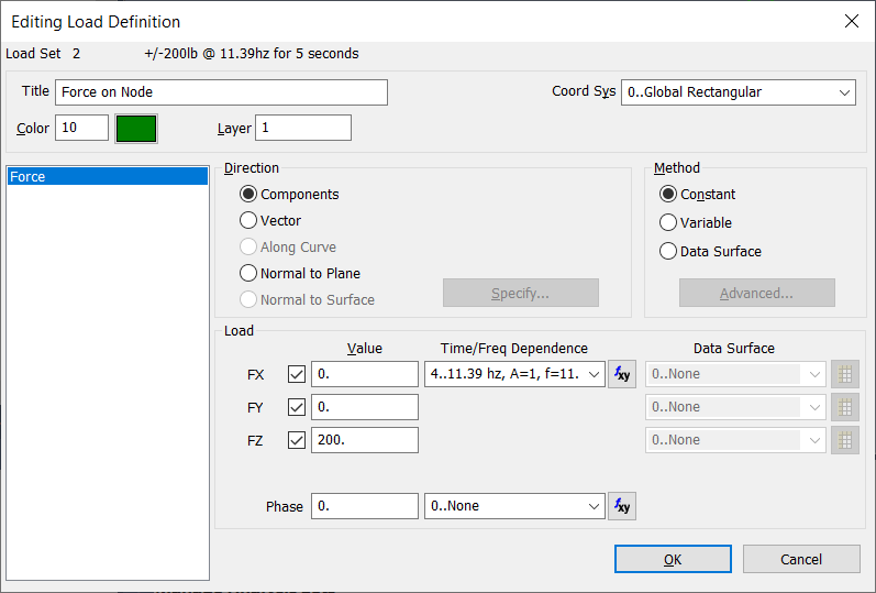
Don’t forget to set Type to 1..vs. Time. One last tip, use the Load Definition that references the function for setting amplitude. It is easier than going back in and adjusting the function. Here, A = 200.